


Investigating the prospect of utilizing evaporative cooling in cities to mitigate the Urban Heat Island Effect
ABSTRACT
Heat islands continue to increase each year as temperatures climb. Urban heat islands increase energy use, degrade water quality, and harm human health by raising temperatures and contributing to heat-related illnesses like heat stroke, dehydration, and respiratory issues. These warmer conditions also promote the growth of bacteria and mosquitoes, increasing the spread of infectious diseases among humans and animals. Many urban areas struggle to manage their temperatures effectively due to heat-absorbing surfaces, a lack of greenery, and gas emissions. In recent years, evaporative cooling has emerged as a potentially efficient and energy-saving approach to lower temperatures in urban areas and mitigate high energy usage in cities. This study aims to assess whether the widespread adoption of evaporative cooling can realistically and effectively mitigate the urban heat island effect in urban settings by more than 7°F. After performing over 6,000 simulations in Google Docs to examine the potential effects, advantages, and costs associated with this approach for both general urban areas and specifically for Houston as a case study, it has been determined that large-scale implementation of evaporative cooling is feasible and advantageous in addressing the urban heat island effect. By applying this strategy, cities can achieve a significant reduction in air temperatures, typically ranging from 6°F to 9°F within the first hour. In hotter conditions, cooling effects are even more substantial, with average decreases between 10°F and 18°F. Implementing this strategy in urban environments could lead to lower electricity usage, healthier aquatic ecosystems, and improved public health, contributing to a more secure living environment. This approach, when combined with other strategies such as cool pavements and green infrastructure, could help pave the way for more sustainable and cooler urban futures.
INTRODUCTION
In recent years, evaporative cooling has emerged as a potentially efficient and energy-saving approach to lower temperatures while also helping to decrease energy consumption in cities [2, 3, 5, 10, 28, 31]. Its current applications span various sectors, including HVAC systems, outdoor cooling, and industrial cooling processes. Researchers regard the potential of utilizing evaporative cooling on a larger scale as a method to mitigate the urban heat island effect [2, 5, 10, 28, 31]. This study aims to evaluate whether the widespread implementation of evaporative cooling can realistically and effectively reduce the urban heat island effect in urban cities.
The urban heat island effect, or UHIE, is a phenomenon where urban areas – heat islands – reach significantly higher temperatures than their surrounding areas. This effect is a result of urbanization, the process through which areas become more crowded and developed, leading to a decrease in greenery and obstruction of airflow [12]. Natural landscapes offer shade and cooling effects that are essential for regulating temperatures, but they are quickly being replaced by heat-retaining surfaces that absorb heat and then re-emit it during cooler hours. This causes temperatures to climb by more than 1-7°F during the day and 2-5°F during the night [23].
Furthermore, numerous towering city structures block natural wind from dispersing heat, causing warm air to build up. Skyscrapers also create a canyon of heat as warm air is funneled into the narrow spaces between tall structures, known as heat funneling, which further retains excess heat [23]. UHIE is trapping urban areas in a dome of heat, and the rising temperatures have already started causing many issues in cities, such as increased energy usage, degradation of water quality, discomfort, and an overall deterioration of human health.
The urban heat island effect leads to a 19% rise in energy usage for cooling relative to surrounding rural or suburban areas, as more air conditioning is required to maintain temperatures inside buildings [9]. The air conditioning units then push out the warm air, further warming the outside atmosphere, which increases the urban heat island effect and creates a never-ending cycle [14]. Cities already use about 19% of their daily electricity on just cooling alone, and with the added impact of UHIE, this number will continue to surge, resulting in a higher demand for electricity from suppliers and a warmer atmosphere [14][21].
The excessively heated pavements caused by UHIE have also started to degrade water quality. Hot pavements raise the temperature of stormwater runoff, which then drains into nearby aquatic ecosystems. The organisms inhabiting these waters struggle to cope with the rising temperatures, resulting in adverse effects on their metabolism and reproductive processes .[30]. According to one study by Zahn et al., urban streams are, on average, 18°F hotter than forested streams after rainfall [30]. This temperature increase leads to a decline in marine life and damages ecosystems, as they cannot adapt to the rapidly increasing temperatures.
UHIE is associated with numerous heat-related illnesses, deaths, and overall deterioration of human health [23]. Excessive heat impairs the body's ability to regulate temperature, and with the urban heat island effect, temperatures will continue to rise beyond what the human body can safely handle, potentially leading to flare-ups from chronic conditions, harming mental health, causing headaches, heat strokes, and impairing concentration [15]. Vulnerable populations such as the elderly, young children, and people in poor health, like those with chronic diseases, disabilities, diabetes, and asthma, are especially susceptible to the extreme rises in temperature, putting them at a greater risk for heat-related complications or even death [6][15]. Moreover, UHIE-induced warming can facilitate the proliferation of non-native bacteria and vectors, thereby altering disease dynamics and increasing the risk of outbreaks among urban populations [13]. This demonstrates how heat-related hospitalizations and deaths will continue to surge as the urban heat island effect becomes more intense and exacerbates the issue further.
CONCEPT
Temperatures near bodies of water tend to be significantly cooler because, as water evaporates, it decreases the temperature of the surface and the surrounding atmosphere. This is a process known as heat vaporization or evaporative cooling. To replicate this process on roads, simply spray cool water onto the heated asphalt. This approach shows potential and may be an efficient means of reducing both surface and air temperatures. By utilizing this technique, cities might lower temperatures by over 7°F simply by spraying water on the roads.
This concept consists of three key components: sourcing, control, and output. Cities can obtain the water needed in several ways by evaluating the geospatial and economic feasibility of primary and secondary sources to aid the system. The water would then be conveyed to the appropriate locations, whether to sub-transporters or directly to the output, preferably using PVC Pipes. When given the command, the water would be applied to the pavement via sprinklers; The water would then evaporate, causing heat vaporization, cooling the pavement and the surrounding atmosphere.
The preferred material for pipes is Polyvinyl Chloride, also known as PVC, which is relatively inexpensive and capable of withstanding high water pressures. These pipes have an impressive lifespan, potentially lasting over 70 years. To effectively manage water pressure, a diameter of 6 or 8 inches is recommended. However, excessive pressure on these pipes can lead to considerable strain. If this type of pipe is selected, it is necessary to reinforce it, which may raise costs.
The sprinklers will rotate a full 360° and have a spraying radius of 10-12 feet, as that’s the average width of a typical road lane. Positioned between the lanes, the sprinkler should efficiently spray the adjacent areas, and if the roadway is wider, excess water will spill over and cover the unsprayed areas as they flow toward the drain. The distance between the sprinklers will be 15-20 feet apart to reduce unsprayed zones. The spray setting is up to the city’s preferences. Still, a gentler and less pressurized spray-like mist would be ideal, as it minimizes excessive back spray that can impair visibility. The sprinklers would operate for 1 to 2 minutes and would reapply water once it is nearly dry.
The sprinkler would be constructed using composite materials that combine both plastic and metal to achieve a balance between cost and durability. A blend of Acrylonitrile Butadiene Styrene (ABS) and Polycarbonate plastic with either brass or stainless steel would be optimal. While Polycarbonate offers high strength and resistance to the elements, ABS plastic is affordable and resistant to impacts, allowing it to withstand blows from cars without shattering; however, it is vulnerable to the weather, making a combination of the two, known as PC/ABS, the best choice. Both brass and stainless steel are suitable options due to their durability.
To gather the data needed to run the concept, turn to the National Weather Forecast (NWF), as it gathers data from governmental satellites, air sampling devices, and weather stations, which is then processed and analyzed at NWF forecast offices to provide localized forecasts. This enables us to have our data organized and filtered, allowing our sprinkler control system to interpret the information and determine when to activate and run the system. If the air temperature reaches 80°F or higher, the system will turn on, as the safe temperature range for prolonged outdoor excursions is 77°F to 88°F, but with urban city conditions (e.g., heat funneling) and the vulnerability of certain groups, the range may be even lower, making 80°F a safer placemarker [6]. The system will cease operation once the air temperature falls below 80°F.
Implementing this design will contribute to a reduction in overall electricity consumption, improve water quality in nearby bodies of water, and minimize health risks associated with heat. With lower air temperatures, the demand for air conditioning will diminish, leading to decreased electricity usage. Pavements will also retain cooler temperatures, which will lower the temperature of runoff water and help maintain a more stable temperature in water bodies. With a decrease in overall atmospheric temperatures, individuals will also face a reduced risk of heat-related health issues, as cooler temperatures will help avoid overheating.
The cost of building this design is influenced by a variety of factors, such as downtown size, pipe material, sprinkler type, design specifications, geographical location, etc. The size of the downtown area is the most significant factor affecting the overall cost of these materials.
METHODS
To test the efficiency, realistic plausibility, and benefits of this concept, a data simulation was run on Google Sheets to discover the statistics of this design. Using publicly available data from national weather websites, a simulation could mimic a city’s geographical weather and climate, giving the impression of a typical day in that location. This simulation could either be tailored to a specific city’s data and geographical weather parameters or serve as a generalization of a specific set of cities with a common variable, such as size.
A key factor in this concept was the city's downtown size, as it influenced numerous aspects. The dimensions of the downtown area dictated the quantity of materials required, which in turn affected the expenses for executing this design. This simulation illustrated the overall projected costs and advantages for smaller downtown areas (0.5 to 1 sq. miles).
To begin, a random temperature was chosen within the range of 80°F to 110°F, representing the unsafe temperature range for prolonged outdoor excursions in cities that suffer from UHIE. Following that, a second random selection was made for a plausible dew point range suitable for urban settings, which spanned from 0°F to 90°F [27]. The estimated length of roads in small downtown areas ranged from 5 to 10 miles, and then wind speed was selected from a range of 0 to 20 MPH, along with solar intensity, which varied between 100 W/m² and 800 W/m². Both wind speed and solar intensity were randomized from a shared range of minimums and maximums for urban locales, due to the high variability in different small downtown regions that made defining a specific range challenging.
With this information, additional factors were determined, including relative humidity and pavement temperature. To find relative humidity, the formula was applied: [8]
e[17.625D(243.04+D)] ÷ e[17.625T(243.04+T)]
e = Euler's number
D = Dew Point(C)
T = Air Temperature(C)
To determine the temperature of asphalt pavement, the following equation was utilized:[7]
26.081-(0.844Ws)+(0.479T)-(0.187RH)-(0.0173Ws)+(0.0042254WsT)+(0.00565WsRH)+(0.0016WsS) +(0.00342TRH)+(0.000117TS)+(5.702910-5RHS) +(0.00425T2+1.912510-5S2
T = Air Temperature (F) S = Solar intensity
Ws = Wind Speed RH = Relative Humidity
Here, wind speed was expressed in MPH, while temperature was measured in degrees Fahrenheit, and solar intensity was measured in W/m².
To determine the efficiency of the system, the evaporation rate was assessed, as it was directly related to the amount of heat that was lost during evaporation. For every gram of water that evaporated, 540 calories of heat were released, which was roughly equivalent to a temperature change of 1°F [3]. To determine the rate of water evaporation in grams per hour, the formula below was used:
(25+19 x Ws) x Sa x (Hm-Hc)
Ws = Windspeed Sa = Surface Area
Hm=Maximum Humidity Hc=Current Humidity
For calculating maximum humidity and current humidity, the following formulas were utilized, respectively: [4]
3.733 x 10^-3 + 3.2 x 10^-4 x T + 3 x 10^-6 x T^2 + 4 x 10^-7 x T^3
T = Temperature©
RH x 0.6113 x e(5423 x (1/273.15 - 1/T) ÷ (461.5 x T)) x 100
RH = Relative Humidity e = Euler's number
T = Temperature(K)
From this, it was deduced that within one hour, the volume of water that evaporated was directly tied to the reduction in temperature, as each gram that evaporated lowered the air temperature by 1°F. By deducting the grams of water that had evaporated from the initial temperature, the atmospheric temperature after one hour was estimated. This simulation was also utilized to estimate the potential variety of materials and associated costs for implementing this concept.
By considering the total miles of road, the required length of piping was determined by converting miles into feet. Similarly, the number of sprinklers was determined by converting miles into feet and dividing by the interval between sprinklers, which was randomly generated within a specific range (15–20 ft.). These calculations enabled the estimation of expenses for the required pipes and sprinklers. The cost for reinforced PVC pipes depended on the diameter of the pipe; thus, by randomly selecting either a 6- or an 8-inch pipe, which were common sizes for water lines, the cost of the pipe was calculated. A reinforced pipe with a 6-inch diameter typically had a market value between $12 and $20, while an 8-inch diameter pipe ranged from $20 to $40. A random number was then generated from the respective cost ranges and multiplied by the total length of pipes needed.
The average market price for a sprinkler head on Amazon fell between $4 and $12, so the total number of sprinklers was multiplied by a randomly selected price from this range to determine the overall sprinkler cost. For the central control system, a cost range of $100,000 to $200,000 was assumed based on typical pricing for industrial-scale control systems that include hardware and software integration [24]. This range reflected variability in system complexity, number of inputs/outputs, and required reliability, and a random value within this interval was used in simulations to account for uncertainty in design specifications and vendor pricing. Additionally, the control system required maintenance, which ranged from $5,000 for a basic data system to $25,000 monthly for a premium system. After calculating all these amounts, they were combined to determine the total material cost, although this calculation did not include the expenses for labor required for installation and maintenance. To estimate the manpower required, the average expense for installing pipes, which ranged from $5 to $20 per foot, was multiplied by the total length of pipes needed [16]. The installation of pipes constituted the majority of the overall labor required, as the costs of the other two materials were either factored into the pipe costs or already included as part of their prices.
Using this information, the overall impacts and advantages of this concept were also assessed. To determine the new relative humidity and pavement temperature, the previous equations were applied, with updated variables such as temperature and relative humidity. However, when calculating pavement temperature, the grams of water evaporated were deducted at the end, since the initial pavement temperature calculation only considered the new variables without accounting for the influence of the system on the pavement, as the evaporation of water also lowered pavement temperatures at a rate of approximately 1°F for every gram of water evaporated [3]. The anticipated benefits were further evaluated by finding the difference between the original inputs and the calculated changes from the concept, including factors such as air temperature, relative humidity, and pavement temperature. Additionally, the reduction in electricity consumption was estimated by multiplying the difference between the initial air temperature and the final air temperature by a randomly generated number ranging from 0.05% to 0.85%, as every 1°F drop in temperature translated to a decrease in electricity demand by 0.05% to 0.85% [26].
To achieve more precise results, customizing the parameters of the simulation to align with an actual urban city allowed for the evaluation of the concept within the specific climate of that city, assisting in a more accurate estimation of the materials and costs if the system was implemented. Taking Houston, TX, as a case study, a simulation was adapted to reflect the city's unique characteristics and climate. The typical low dew point in Houston was approximately 50°F, while the typical high was around 75°F [22]. By allowing for a variance of 15°F, it was inferred that Houston's average dew point spanned from 35°F to 90°F. Additionally, Houston experienced less wind compared to many other urban cities, with wind speeds ranging from 0 to 12 MPH throughout the year [29].
The solar intensity in Houston was somewhat milder than that of other cities, but only slightly, reducing the range to about 100 to 700 W/m² [29]. By focusing on a particular city, a more precise estimation of the costs and materials needed was achieved, given that a fixed measurement of the miles of road in the downtown area was established. However, this information was not publicly accessible, so an estimation of the total miles of road in Houston was required. Downtown Houston covered roughly 1.84 square miles (4.8 km²) and was bordered by Interstate 10, Interstate 45, and Interstate 69 [22]. This area included about 400 square blocks, each measuring approximately 250 × 250 feet. Twenty rows of blocks required 21 horizontal streets, and the 20 columns of blocks required 21 vertical streets. However, considering double blocks and larger spaces that accounted for around 15% of Houston, the calculation was adjusted to approximately 85% of the original count, yielding about 17 rows and 17 columns. This reduced the total number of individual roads to 18 horizontal and 18 vertical roads. Each block was approximately 250 feet on each side. The horizontal and vertical roads spanned a length of about 20 blocks, resulting in each road measuring around 5,000 feet. By multiplying this by the 36 separate roads, a total of 153,000 feet of roads was obtained, which converted to about 29 miles, indicating that downtown Houston had roughly 29 miles of road.
Using this approach, a precise cost range estimate for Houston, TX, was determined, along with all the other parameters mentioned earlier. This technique could also be utilized in various urban areas to obtain more precise data on the estimated advantages, costs, and other factors relevant to the specific climate and circumstances of those cities.
RESULTS
After conducting over 6,000 simulations to analyze the potential impacts, benefits, and costs of the concept for both general small cities and Houston, mass-scale use of evaporative cooling for cities is realistically feasible and beneficial in mitigating the urban heat island effect.
In general cities, the concept is shown to decrease temperatures by, on average, 7.93°F after one hour. Additionally, the pavement temperature decreases by, on average, 18.64°F, and the concept reduces the demand for electric heating by 35.80%. The approach also resulted in an average increase in relative humidity of 7.41% during the first hour, which may affect the atmosphere and pedestrian comfort if used in high-humidity areas. However, the system becomes less effective as temperatures drop, leading to a reduction in its cooling capacity over time.
During the first hour, the average temperature reduction was 7.93°F, while the second hour saw an average drop of 5.68°F, followed by a decrease of 4.52°F in the third hour, and the temperature reduction rate continued decreasing over time, with the 4th hour’s decrease being a 4.22°F drop and the 5th hour being a 3.49°F drop. This pattern is similarly observed in pavement temperatures, with the initial hour recording a higher reduction of 18.64°F, then 5.21°F in the second hour, and 4.30°F in the third hour. Though the temperature reduction slightly increased during the fourth hour to an average of 4.89°F, before declining again during the fifth hour, averaging a reduction of 3.39°F. The rise in relative humidity also varies, starting with an average increase of 7.41% in the first hour, followed by 5.04% in the second, 9.26% in the third, and 7.28% in the fourth and fifth hours.
The average total for materials amounted to $1,235,193, including $1,066,570 for pipes, $18,466 for sprinklers, and $150,156 for the control system. When factoring in installation labor costs, the average total rises to $24,218,009, with labor expenses averaging $26,358,415.
In Houston, the concept results in an average temperature reduction of 5.09°F after one hour. On average, the pavement temperature sees a decrease of 12.03°F, and the demand for cooling electricity decreases by 23.01%. Additionally, there is an average increase in relative humidity of 6.03%. The system's effectiveness is lower in Houston’s climate, with less significant temperature reductions.
Houston’s results closely resemble the earlier simulations conducted for general urban cities, with an average temperature drop of 5.09°F in the first hour. In the second hour, the temperature decrease is 4.13°F, followed by a 3.49°F drop in the third hour, 3.25°F in the fourth hour, and a 2.83°F drop in the fifth hour; this trend of decreasing temperature drops continues over time. A similar pattern is observed in pavement temperatures, where the average drop is 12.03°F in the first hour, followed by a 4.45°F decrease in the second hour and a 3.75°F drop during the third hour. The reduction in temperature increases to an average of 3.34°F during the fourth hour, then resumes its decline in the fifth hour with an average decrease of 3.04°F. Relative Humidity increases without a clear pattern, starting with a rise of 6.03% in the first hour, another 6.03% increase in the second hour, a 5.96% rise in the third hour, a 6.08% rise in the fourth hour, and a 6.1% increase in the fifth hour. The Relative Humidity consistently rises by a similar percentage each hour, exhibiting little variation.
For Houston, the average total expense for materials was $4,114,075, which included $3,892,772 for pipes, $70,565 for sprinklers, and an average of $150,738 for the control system. When factoring in installation labor costs, the average overall expense would reach $52,145,893, with labor costs averaging around $48,031,849. This table displays the average, highest, and lowest costs for each variable.


DISCUSSION
The findings indicate that in most urban areas, the system effectively lowers air and pavement temperatures while decreasing electricity consumption. Nevertheless, the cooling effect diminishes over time, and humidity levels increase, potentially affecting comfort in humid regions. In Houston, the system proves to be less effective because of the local climate, with its higher average humidity. It still achieves a reduction in temperatures and energy use, but not to the extent seen in typical cities. The cooling effect consistently declines over time, while humidity progressively rises at a steady pace.
These results show that the mass-scale use of evaporative cooling for cities is realistically plausible and beneficial in decreasing the urban heat island effect. By adopting this approach, cities can experience a notable reduction in air temperatures, with decreases typically ranging from 6°F to 9°F during the first hour. In situations with higher temperatures, the cooling is even more pronounced, with average reductions between 10°F and 18°F. Such decreases in air temperature could significantly lower the incidence of heat-related health issues and fatalities, while also fostering a more pleasant environment for city residents. However, the extent of this temperature reduction can vary based on the local climate, as specific conditions may influence the system’s efficiency. This was evident in the simulations conducted for Houston, where the city experienced less effective cooling compared to the typical urban scenario due to its high humidity, which hampers the water evaporation process.
Along with air temperature, pavement temperature decreased by an average range of 12°F to 19°F. With lower pavement temperatures, nearby aquatic organisms will no longer be impacted by heated runoff, enabling their metabolism and reproduction to stabilize once again. Additionally, this will help prevent pavements from rising to potentially hazardous temperatures that could lead to severe burns for pets, humans, and other animals.
While a few of these graphs indicate that the relative humidity exceeds 100%, this is improbable because of the presence of other particles in the atmosphere. The simulations overlooked this factor, making certain scenarios quite unlikely to happen in reality. Furthermore, many simulations continued cooling despite the atmosphere temperature going below 80°F, as the simulations weren't run with a killswitch, causing the relative humidity to skyrocket towards the end of the simulations. (Figure 5, 6)
The demand for electricity for cooling was reduced by an average range of 23% to 36% with this concept. This can save a city copious amounts of electricity and reduce the strain on systems during high-heat months, as cooling represents the highest electricity consumption during summer, accounting for 19% of total electricity usage in urban areas. [20]
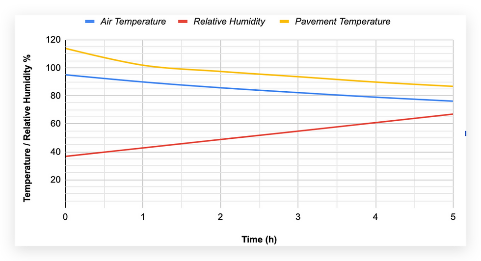


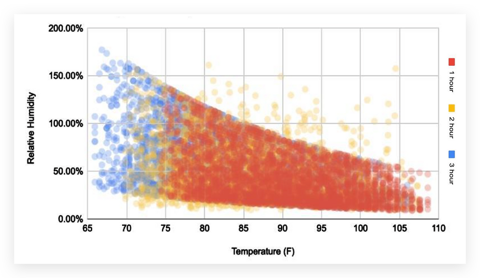
As time goes on, the effectiveness of these processes diminishes since the lower temperatures hinder the rate of water evaporation, resulting in progressively smaller temperature drops with each hour. This effect has minimal impact on the increase in relative humidity, which consistently rises by 7% to 9% during the overall simulation without following a clear pattern. However, the increase in Relative Humidity is influenced by a city's climate; for example, in Houston, the Relative Humidity rise remains between an average of 5.9% to 6.1% throughout all hours, indicating that variations in relative humidity increases can occur based on the specific characteristics of different cities.
This could pose a challenge in regions with elevated humidity, as the idea might exacerbate the moisture levels to an intolerable extent. This is particularly evident during the later hours of the simulation when the reduction in air and pavement temperatures has considerably slowed, while the Relative Humidity continues to increase steadily. At this stage, the concept fails to fulfill its initial objective of cooling and instead fosters a humid environment that, if sustained for a prolonged period, may entirely negate the original cooling effect.
Therefore, it is advisable to approach this concept with caution in areas with high humidity levels. Conversely, this concept could introduce essential humidity and create a more moist atmosphere in cities characterized by arid climates.


The expense of implementing this concept differs significantly based on the city’s size. The larger the city, the more materials you’ll need to build the system. However, the most expensive aspect of implementation is the labor, accounting for approximately 91.88% of the total cost in general urban areas, and 92.11% in Houston specifically. The materials constitute less than 10% of the overall expense, with pipes accounting for 7.42%, sprinklers at 0.14%, and the control facility at 0.57%. In Houston, these figures are 7.47%, 0.14%, and 0.29%, respectively. The cost of the control system remains relatively stable, meaning that as the total cost increases, the percentage it represents of the overall expenses decreases. The costs of other materials increase with the size of the downtown area, resulting in their percentage costs remaining in a similar range. Therefore, the overall expense heavily relies on labor costs, as wages differ from city to city, significantly influencing the total cost of the concept.
Every urban city has its distinct climate, which means that applying this in a specific city will require additional research and time to customize the simulation’s parameters to match the local climate conditions. Additionally, there are numerous factors beyond those incorporated into this simulation, such as the influence of shade and vehicle coverage on evaporation rates, which could affect the effectiveness of this concept. Many other minor factors were not included in these simulations that might impact the concept in either a positive or negative way.
The simulations featured calculations that were not entirely reflective of real-world scenarios, as other factors may fluctuate over time; these variations were not included in the simulation and were instead treated as constants. The results merely illustrate the system's impact without accounting for any variations in other factors, such as wind speed and solar radiation. This does not align with real life, as these parameters are continually changing, so to attain more precise results, the simulation would need to continuously monitor potential wind patterns and other parameters.
Should this concept be applied in an urban environment, extensive additional testing would be required to determine its suitability for the specific city's climate, since this concept may not be ideal for every city. Some attributes of a city might render the system ineffective or even harmful, particularly in areas with elevated humidity levels.
CONCLUSION
This study shows that the widespread implementation of evaporative cooling can realistically and effectively mitigate the urban heat island effect in urban environments. The findings from the simulations indicate that large-scale evaporative cooling systems can significantly lower temperatures and decrease energy consumption in urban locations, making them effective in combating the urban heat island effect. However, over time, the cooling benefits began to lessen, accompanied by a steady rise in humidity. In conclusion, although the efficiency of this method declines over time and the implementation costs are relatively high, this cooling strategy holds promise due to its distinct mechanism. This approach could be combined with other techniques to help eliminate the urban heat island effect.
ACKNOWLEDGMENTS
I would like to express my deepest gratitude to Ms. Heather Domjan from Houston University, as this paper would have never happened without her. I would also like to thank Dr. Andrew Karpral for their invaluable guidance and insightful feedback throughout this research project. Lastly, I want to thank Ms. Valeria Servin for her support through the revisions of this paper, as well as being the first person to read my paper in full and provide feedback.
WORKS CITED
Ali, Muhammad, and Muhammad Abidin. “Population Density and Intensity of Traffic Connection: Spatial Analysis (Overlay).” International Journal of Science and Research (IJSR), vol. 7, no. 12, Dec. 2018, pp. 546–52. DOI:10.31227/osf.io/v4dq8.
Chen, Han, et al. “Revealing the Response of Urban Heat Island Effect to Water Body Evaporation from Main Urban and Suburb Areas.” Journal of Hydrology, vol. 623, 1 Aug. 2023, p. 129687, www.sciencedirect.com/science/article/pii/S0022169423006297, https://doi.org/10.1016/j.jhydrol.2023.129687
Cheng, Wen-long. “Spray cooling and flash evaporation cooling: The current development and application.” Renewable and Sustainable Energy Reviews, vol. 55, Mar. 2016, pp. 614–28. https://doi.org/10.1016/j.rser.2015.11.014.
Huang, Jianhua. “A Simple Accurate Formula for Calculating Saturation Vapor Pressure of Water and Ice.” Journal of Applied Meteorology and Climatology, vol. 57, no. 6, 1 June 2018, pp. 1265–72. https://doi.org/10.1175/JAMC-D-17-0334.1.
Jandaghian, Zahra, and Andrew Colombo. “The Role of Water Bodies in Climate Regulation: Insights from Recent Studies on Urban Heat Island Mitigation.” Buildings, vol. 14, no. 9, 18 Sept. 2024, p. 2945, https://doi.org/10.3390/buildings14092945.
Johannesson, Inga. “What Temperature Is Too Hot for Humans? Understanding Heat Index.” GoodRx, 6 Aug. 2024, www.goodrx.com/health-topic/environmental/temperature-too-hot-for-humans#.
Khan, Zafrul, et al. “Determining asphalt surface temperature using weather parameters.” Journal of Traffic and Transportation Engineering, vol. 6, no. 6, Dec. 2019, pp. 577–88. https://doi.org/10.1016/j.jtte.2018.04.005.
Lawrence, Mark. “The Relationship between Relative Humidity and the Dewpoint Temperature in Moist Air: A Simple Conversion and Applications.” Bulletin of the American Meteorological Society, vol. 86, no. 2, 1 Feb. 2005, pp. 225–34. https://doi.org/10.1175/BAMS-86-2-225.
Li, Xiaoma, et al. “Urban heat island impacts on building energy consumption: A review of approaches and findings.” Energy, vol. 174, 1 May 2019, pp. 407–19. https://doi.org/10.1016/j.energy.2019.02.183.
Liu, Shiyong, et al. “The Design of an Urban Roadside Automatic Sprinkling System: Mitigation of PM2.5–10 in Ambient Air in Megacities.” Chinese Journal of Engineering, vol. 2014, 23 July 2014, article no. 618109. https://doi.org/10.1155/2014/618109.
Qin, Yinhong, et al. “A new water-retaining paver block for reducing runoff and cooling pavement.” Journal of Cleaner Production, vol. 199, 20 Oct. 2018, pp. 948–56. https://doi.org/10.1016/j.jclepro.2018.07.250.
Rani, T. “Urban Heat Island: Causes, impact and damage control measures.” Journal of Interior Designing and Regional Planning, vol. 7, no. 3, 17 Sept. 2024, pp. 1–12. https://doi.org/10.5281/zenodo.13772289.
Rohr, Jason R., and Jeremy M. Cohen. “Understanding How Temperature Shifts Could Impact Infectious Disease.” PLOS Biology, vol. 18, no. 11, 24 Nov. 2020, p. e3000938, https://doi.org/10.1371/journal.pbio.3000938.
Santamouris, Matteos. “On the impact of urban heat island and global warming on the power demand and electricity consumption of buildings—A review.” Energy and Buildings, vol. 98, 1 July 2015, pp. 119–24. https://doi.org/10.1016/j.enbuild.2014.09.052.
United States, Centers for Disease Control and Prevention, Morbidity and Mortality Weekly Report. Vaidyanathan, Ambarish, et al. “Heat-Related Deaths — United States, 2004–2018.” MMWR Morb Mortal Wkly Rep, 19 June 2020. https://www.cdc.gov/mmwr/volumes/69/wr/mm6924a1.htm.
United States, Department of Transportation. “Phases of Pipeline Construction: An Overview. Pipeline and Hazardous Materials Safety Administration.” 18 Apr. 2022. https://www.phmsa.dot.gov/technical-resources/pipeline/pipeline-construction/phases-pipeline-construction-overview.
United States, Department of Transportation, Federal Highway Administration. “How Do Weather Events Impact Roads?” 6 Sept. 2024. https://ops.fhwa.dot.gov/weather/q1_roadimpact.htm#
United States, Department of Transportation, Federal Highway Administration. “Rain and Flooding.” 6 Sept. 2024. https://ops.fhwa.dot.gov/weather/weather_events/rain_flooding.htm#
United States, Energy Information Administration. “Electricity explained, Use of electricity.” 2022. https://www.eia.gov/energyexplained/electricity/use-of-electricity.php.
United States, Energy Information Administration. “Hourly electricity consumption varies throughout the day and across seasons.” 21 Feb. 2020. https://www.eia.gov/todayinenergy/detail.php?id=42915.
United States, Energy Information Administration. “How much electricity is used for air conditioning in the United States?” 15 Mar. 2024. https://www.eia.gov/tools/faqs/faq.php?id=1174&t=1.
United States, Environmental Protection Agency. “EPA Urban Heat Island Pilot Project City Profile: Houston.” 1998–2002. https://19january2017snapshot.epa.gov/sites/production/files/2014-08/documents/houston.pdf.
United States, Environmental Protection Agency. “Heat Island Effect.” 2022. https://www.epa.gov/heatislands.
United States, Environmental Protection Agency. “Particulate Matter (PM) Pollution.” 4 Sept. 2024. https://www.epa.gov/pm-pollution.
United States, National Institute of Standards and Technology, Department of Commerce. “How Do You Measure Air Temperature Accurately?” 13 Apr. 2022. https://www.nist.gov/how-do-you-measure-it/how-do-you-measure-air-temperature-accurately#
United States, NYC Open Data. “Electric Consumption And Cost (2010 - Feb 2023).” 11 Apr. 2023. https://data.cityofnewyork.us/Housing-Development/Electric-Consumption-And-Cost-2010-Feb-2023-/jr24-e7cr/about_data.
United States, University of Miami. “Heat Index and DewPoint Climatology for Houston, TX.” 1948–14 July 2024. https://bmcnoldy.earth.miami.edu/hou/.
Wang, Yasha, and Wanlu Ouyang. “Investigating the heterogeneity of water cooling effect for cooler cities.” Sustainable Cities and Society, vol. 35, Dec. 2021, article no. 103281. https://doi.org/10.1016/j.scs.2021.103281.
“Houston Climate, Weather by Month, Average Temperature (Texas, United States) - Weather Spark.” Weatherspark.com, weatherspark.com/y/9247/Average-Weather-in-Houston-Texas-United-States-Year-Round.
Zahn, Einara, et al. “The Hydrological Urban Heat Island: Determinants of Acute and Chronic Heat Stress in Urban Streams.” Journal of the American Water Resources Association, vol. 57, no. 6, 31 Oct. 2021, pp. 941–55. https://doi.org/10.1111/1752-1688.12963.
Zhu, Dun, et al. “Water Effects on Urban Heat Islands in Summer Using WRF-UCM with Gridded Urban Canopy Parameters — a Case Study of Wuhan.” Building and Environment, vol. 225, Nov. 2022, p. 109528, https://doi.org/10.1016/j.buildenv.2022.109528.
Mordor Intelligence. “North America Factory Automation & Industrial Controls Market - Size & Share.” Mordor Intelligence, 16 Jan. 2026, www.mordorintelligence.com/industry-reports/north-america-factory-automation-and-industrial-controls-market. Accessed 25 Apr. 2026.



Comments